


Next: Arc Length and Curvature Up: Three Dimensional Geometry Previous: Lines, Planes, and Quadric Contents
We define vector functions in Maxima just like we would any other function; the only difference is that the return value is a vector.
![\begin{maximasession}
r(t) := [t, cos(t), sin(t)];
\maximaoutput*
\i1. r(t) := [...
...t(t\right)\mathbin{:=}\left[ t , \cos t , \sin t \right] \\
\end{maximasession}](img49.png)
Once we have the function we can plug in values of t to evaluate.
![\begin{maximasession}
r(1);
float(%);
\maximaoutput*
\i2. r(1); \\
\o2. \left[ ...
...eft[ 1.0 , .5403023058681398 , .8414709848078965 \right] \\
\end{maximasession}](img50.png)
Now let's try some plotting. Let's first try a space curve of the vector function. We need the draw package to make this happen. Once we have it loaded, we do space curves with the parametric function inside of a draw command.
![\begin{maximasession}
load(draw);
draw3d(parametric(cos(t), -cos(t), sin(t), t, ...
...t[ \mathrm{gr3d}\left(\mathrm{parametric}\right) \right] \\
\end{maximasession}](img51.png)
See Figure 1. Sometimes the line width of a space curve leaves something to be desired. We can fix the issue with the line width argument to the draw command. See Figure 2.
Limits of vector functions operate just like limits of everything else. Notice below how to do limits from the right and left.
![\begin{maximasession}
limit(r(t), t, 2);
float(%);
limit(r(t), t, 2, plus);
limi...
..., 3, minus); \\
\o9. \left[ 3 , \cos 3 , \sin 3 \right] \\
\end{maximasession}](img53.png)
Derivatives of vector-valued functions are, again, just like their one-valued counterparts.
![\begin{maximasession}
diff(r(t), t);
\maximaoutput*
\i10. diff(r(t), t); \\
\o10. \left[ 1 , -\sin t , \cos t \right] \\
\end{maximasession}](img54.png)
We need to be careful, here. In both Maple and Maxima the return value of diff(r(t),t) is an expression, and is NOT a function (although it sure does look like one). Looks are deceptive in this case. Watch what happens if we try to use it like a function.
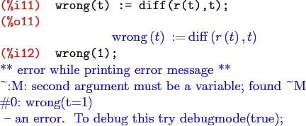
This is not right. The way to get around this in Maple is to do D(r(t),t), and the way to get around this in Maxima is to do the following.
![\begin{maximasession}
define(rp(t), diff(r(t), t));
\maximaoutput*
\i13. define(...
...(t\right)\mathbin{:=}\left[ 1 , -\sin t , \cos t \right] \\
\end{maximasession}](img56.png)
Now we get what we expect.
![\begin{maximasession}
float(rp(1));
\maximaoutput*
\i14. float(rp(1)); \\
\o14....
...ft[ 1.0 , -.8414709848078965 , .5403023058681398 \right] \\
\end{maximasession}](img57.png)
We may define the unit tangent vector  as the normalized derivative of
  . We do this with the uvect function in the eigen package.
![\begin{maximasession}
load(eigen);
uvect(rp(t));
trigsimp(%);
define(T(t), %);
\...
...n t}\over{\sqrt{2}}} , {{\cos t}\over{\sqrt{2}}} \right] \\
\end{maximasession}](img60.png)
To get the unit normal vector we need to get the derivative of and normalize.
![\begin{maximasession}
define(Tp(t), diff(T(t), t));
\maximaoutput*
\i19. define(...
... t}\over{\sqrt{2}}} , -{{\sin t}\over{\sqrt{2}}} \right] \\
\end{maximasession}](img61.png)
![\begin{maximasession}
uvect(Tp(t));
trigsimp(%);
define(N(t), %);
\maximaoutput*...
...t\right)\mathbin{:=}\left[ 0 , -\cos t , -\sin t \right] \\
\end{maximasession}](img62.png)
Now we find the binormal vector,  , by calculating the cross product of and
  . Remember to do load(vect) if you haven't already during the session.
![\begin{maximasession}
load(vect);
express(T(t) N(t));
trigsimp(%);
define(B(t)...
... t}\over{\sqrt{2}}} , -{{\cos t}\over{\sqrt{2}}} \right] \\
\end{maximasession}](img65.png)
![\begin{maximasession}
float(B(1));
\maximaoutput*
\i27. float(B(1)); \\
\o27. \...
...1865475 , .5950098395293859 , -.3820514243700898 \right] \\
\end{maximasession}](img66.png)
