Lines, Planes, and Quadric Surfaces

We can plot planes with implicitplot from the draw package.

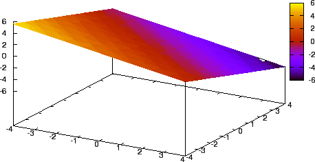
First let us define the plane with equation

$$3x + 4y + 5z = 0.$$

We store the equation of the plane in the variable plane1.

Figure 1: A plot of a plane

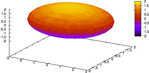
Let us next plot an ellipsoid with equation

$$\frac{x^2}{3} + y^2 + z^2 = 3.$$

We plot it just like we plot the plane.

Figure 2: A plot of an ellipsoid

We can also use Maxima to help us find an equation of a plane based on defining vectors. For instance, let's find and plot the plane determined by the points $A(1,1,1)$, $B(1,2,3)$, and $C(0,0,0)$.

First we define the position vectors for the three defining points.

Next, we find the vectors from $A$ to $B$, and $A$ to $C$.

Then, we find the normal vector to the plane. (Recall that we need the vect package to do cross products.)

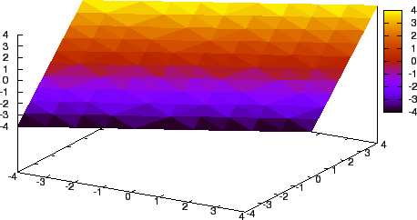
Finally, we set up the defining equation of the plane, which takes the form

$$\mathbf{n}\cdot\mathbf{r} = \mathbf{n}\cdot\mathbf{r_0}.$$

The only remaining task is to make the plot. See Figure BLANK.

Figure 3: Another plot of a plane

We can do more exotic plots, like cones. Let's do a standard cone with equation

$$x^2 + y^2 = z^2$$

Figure 4: A plot of a cone

See Figure BLANK. See how the center of the cone looks distorted? It is because we are plotting the cone in rectangular coordinates. We get a much better plot with spherical coordinates. More on that later.

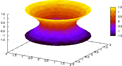
Let's next try a hyperboloid with equation

$$x^2 + y^2 - z^2 = 1$$

See Figure BLANK.

Figure 5: A plot of a hyperboloid

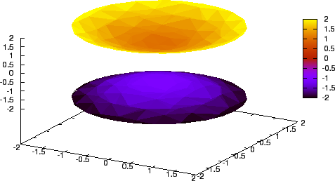
And we can do a hyperboloid of two sheets, with the equation

$$-x^2 - y^2 + z^2 = 1.$$

See Figure BLANK.

Figure 6: Another plot of a hyperboloid