Next: Miscellaneous Up: Vector Calculus Previous: Of vector fields Contents
We know from theory that a vector field ![]() is conservative if there exists a function
is conservative if there exists a function ![]() such that
such that
![]() . Further, we know that fields defined on suitably nice regions are conservative if they are irrotational.
. Further, we know that fields defined on suitably nice regions are conservative if they are irrotational.
We can check whether a field is conservative with the curl function in the vect package. For example, let's check the field
![]() .
.
![\begin{maximasession}
F(x,y) := [4*x^3 - 5*y^2, 5*y^3 - 3*x];
load(vect);
scalef...
...x^3-5\,y^2\right) \\
\i6. ev(%, diff); \\
\o6. 10\,y-3 \\
\end{maximasession}](img228.png)
Since the curl is not zero, the field is not conservative. How about
![\begin{maximasession}
F(x,y) := [x^3 + 5*y, 5*y^3 + 5*x];
ev(express(curl(F(x,y)...
...ht] \\
\i8. ev(express(curl(F(x,y))), diff); \\
\o8. 0 \\
\end{maximasession}](img230.png)
Since the curl is zero, this field is conservative. So the function ![]() satisfying
satisfying
![]() exists. We can find the scalar potential
exists. We can find the scalar potential ![]() in Maxima with the potential function (also in the vect package).
in Maxima with the potential function (also in the vect package).
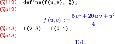
Note, however, that because of a bug in Maxima at the time of this writing we need to do a little fancy footwork. We cannot use the letter x in the function call; instead we will change it to another letter. When we do that, we must follow it by a call to scalefactors.
![\begin{maximasession}
F(u,v) := [u^3 + 5*v, 5*v^3 + 5*u];
scalefactors([u,v]);
p...
...ntial(F(u,v)); \\
\o11. {{5\,v^4+20\,u\,v+u^4}\over{4}} \\
\end{maximasession}](img231.png)
We can easily check that
![]() satisfies
satisfies
![]() . The fundamental theorem for line integrals now allows us to compute line integrals that look like
. The fundamental theorem for line integrals now allows us to compute line integrals that look like
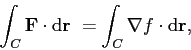
![\begin{displaymath}
\int_C\mathbf{F}\cdot\mathrm{d}\mathbf{r} =
\int_C \left[(x...
...f{i} + (5y^3 + 5x)\mathbf{j} \right] \cdot\mathrm{d}\mathbf{r}
\end{displaymath}](img236.png)
All of the above can be done in three dimensions, too. We need only to do scalefactors([x,y,z]) and scalefactors([u,v,w]), when appropriate.
G. Jay Kerns 2009-12-01